Stack
- Stack is an ordered list in which, insertion and deletion can be performed only at one end that is called top.
- Stack is a recursive data structure having pointer to its top element.
- Stacks are sometimes called as Last-In-First-Out (LIFO) lists i.e. the element which is inserted first in the stack, will be deleted last from the stack.
Applications of Stack
- Recursion
- Expression evaluations and conversions
- Parsing
- Browsers
- Editors
- Tree Traversals
Operations on Stack
There are various operations which can be performed on stack.
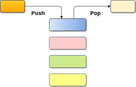
1. Push : Adding an element onto the stack
Stack
- Stack is an ordered list in which, insertion and deletion can be performed only at one end that is called top.
- Stack is a recursive data structure having pointer to its top element.
- Stacks are sometimes called as Last-In-First-Out (LIFO) lists i.e. the element which is inserted first in the stack, will be deleted last from the stack.
Applications of Stack
- Recursion
- Expression evaluations and conversions
- Parsing
- Browsers
- Editors
- Tree Traversals
Operations on Stack
There are various operations which can be performed on stack.
1. Push : Adding an element onto the stack
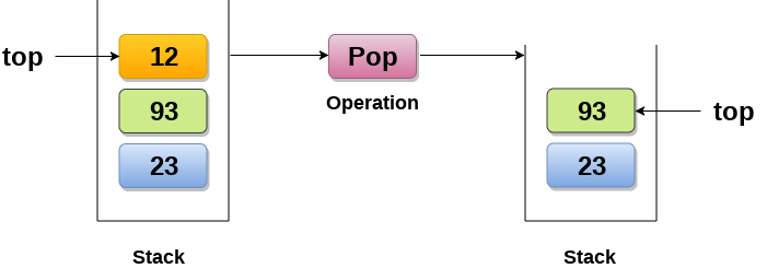
2. Pop : Removing an element from the stack
3. Peek : Look all the elements of stack without removing them.
How the stack grows?
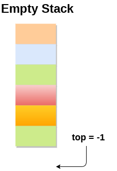
Scenario 1 : Stack is empty
The stack is called empty if it doesn't contain any element inside it. At this stage, the value of variable top is -1.
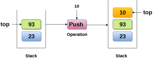
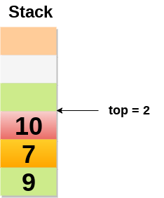
Scenario 2 : Stack is not empty
Value of top will get increased by 1 every time when we add any element to the stack. In the following stack, After adding first element, top = 2.
Scenario 3 : Deletion of an element
Value of top will get decreased by 1 whenever an element is deleted from the stack.
In the following stack, after deleting 10 from the stack, top = 1.

Top and its value :
Top position Status of stack -1 Empty 0 Only one element in the stack N-1 Stack is full N Overflow Array implementation of Stack
In array implementation, the stack is formed by using the array. All the operations regarding the stack are performed using arrays. Lets see how each operation can be implemented on the stack using array data structure.
Adding an element onto the stack (push operation)
Adding an element into the top of the stack is referred to as push operation. Push operation involves following two steps.
- Increment the variable Top so that it can now refere to the next memory location.
- Add element at the position of incremented top. This is referred to as adding new element at the top of the stack.
Algorithm:
Time Complexity : o(1)
implementation of push algorithm in C language
Deletion of an element from a stack (Pop operation)
Deletion of an element from the top of the stack is called pop operation. The value of the variable top will be incremented by 1 whenever an item is deleted from the stack. The top most element of the stack is stored in an another variable and then the top is decremented by 1. the operation returns the deleted value that was stored in another variable as the result.
The underflow condition occurs when we try to delete an element from an already empty stack.
Algorithm :
Time Complexity : o(1)
Implementation of POP algorithm using C language
Visiting each element of the stack (Peek operation)
Peek operation involves returning the element which is present at the top of the stack without deleting it. Underflow condition can occur if we try to return the top element in an already empty stack.
Algorithm :
PEEK (STACK, TOP)
Time complexity: o(n)
Implementation of Peek algorithm in C language
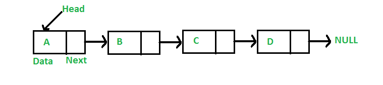
Linked list implementation of stack
Instead of using array, we can also use linked list to implement stack. Linked list allocates the memory dynamically. However, time complexity in both the scenario is same for all the operations i.e. push, pop and peek.
In linked list implementation of stack, the nodes are maintained non-contiguously in the memory. Each node contains a pointer to its immediate successor node in the stack. Stack is said to be overflown if the space left in the memory heap is not enough to create a node.
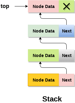
The top most node in the stack always contains null in its address field. Lets discuss the way in which, each operation is performed in linked list implementation of stack.
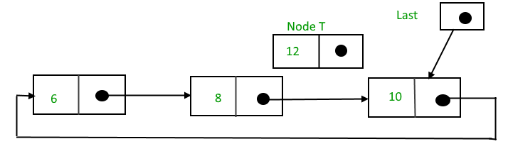
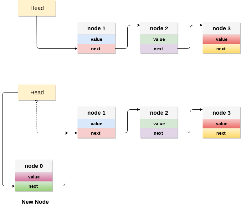
Adding a node to the stack (Push operation)
Adding a node to the stack is referred to as push operation. Pushing an element to a stack in linked list implementation is different from that of an array implementation. In order to push an element onto the stack, the following steps are involved.
- Create a node first and allocate memory to it.
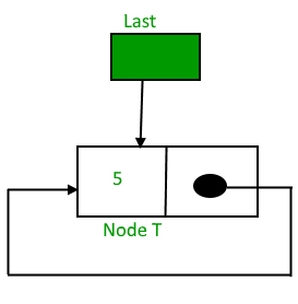
- If the list is empty then the item is to be pushed as the start node of the list. This includes assigning value to the data part of the node and assign null to the address part of the node.
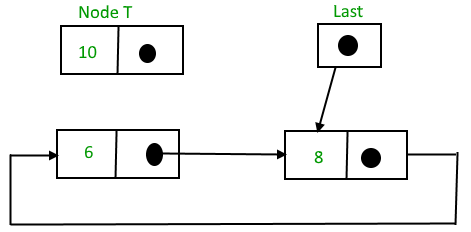
- If there are some nodes in the list already, then we have to add the new element in the beginning of the list (to not violate the property of the stack). For this purpose, assign the address of the starting element to the address field of the new node and make the new node, the starting node of the list. Time Complexity : o(1)
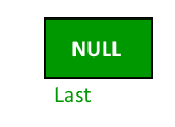
- Check for the underflow condition: The underflow condition occurs when we try to pop from an already empty stack. The stack will be empty if the head pointer of the list points to null.
- Adjust the head pointer accordingly: In stack, the elements are popped only from one end, therefore, the value stored in the head pointer must be deleted and the node must be freed. The next node of the head node now becomes the head node.
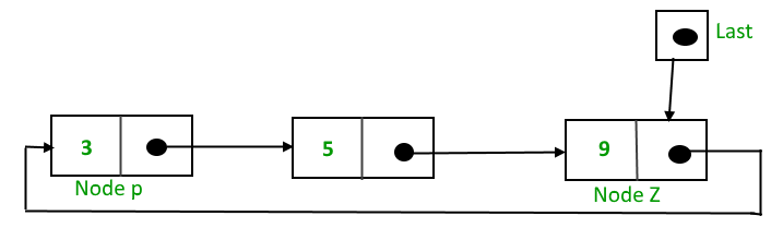
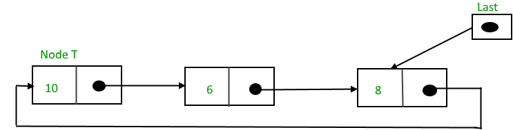
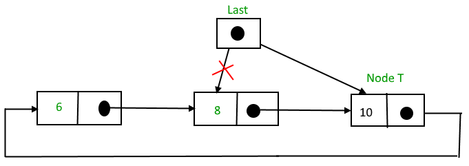
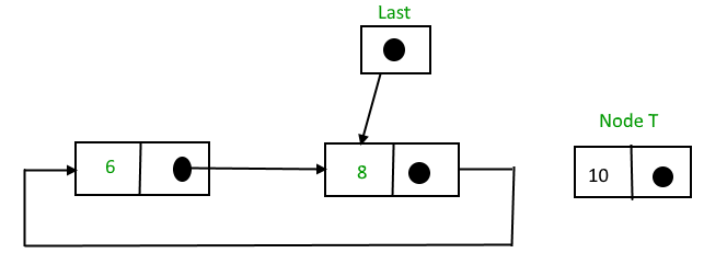
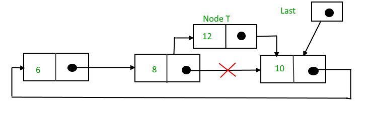
Deleting a node from the stack (POP operation)
Deleting a node from the top of stack is referred to as pop operation. Deleting a node from the linked list implementation of stack is different from that in the array implementation. In order to pop an element from the stack, we need to follow the following steps :Queue
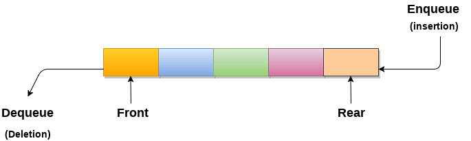
1. A queue can be defined as an ordered list which enables insert operations to be performed at one end called REAR and delete operations to be performed at another end called FRONT.
2. Queue is referred to be as First In First Out list.
3. For example, people waiting in line for a rail ticket form a queue.
Applications of Queue
Due to the fact that queue performs actions on first in first out basis which is quite fair for the ordering of actions. There are various applications of queues discussed as below.
- Queues are widely used as waiting lists for a single shared resource like printer, disk, CPU.
- Queues are used in asynchronous transfer of data (where data is not being transferred at the same rate between two processes) for eg. pipes, file IO, sockets.
- Queues are used as buffers in most of the applications like MP3 media player, CD player, etc.
- Queue are used to maintain the play list in media players in order to add and remove the songs from the play-list.
- Queues are used in operating systems for handling interrupts.
Array representation of Queue
We can easily represent queue by using linear arrays. There are two variables i.e. front and rear, that are implemented in the case of every queue. Front and rear variables point to the position from where insertions and deletions are performed in a queue. Initially, the value of front and queue is -1 which represents an empty queue. Array representation of a queue containing 5 elements along with the respective values of front and rear, is shown in the following figure.
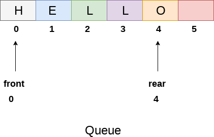
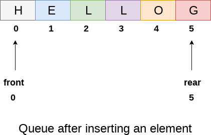
The above figure shows the queue of characters forming the English word "HELLO". Since, No deletion is performed in the queue till now, therefore the value of front remains -1 . However, the value of rear increases by one every time an insertion is performed in the queue. After inserting an element into the queue shown in the above figure, the queue will look something like following. The value of rear will become 5 while the value of front remains same.
Algorithm to insert any element in a queue
Check if the queue is already full by comparing rear to max - 1. if so, then return an overflow error.
If the item is to be inserted as the first element in the list, in that case set the value of front and rear to 0 and insert the element at the rear end.
Otherwise keep increasing the value of rear and insert each element one by one having rear as the index.
Algorithm
- Step 1: IF REAR = MAX - 1
Write OVERFLOW
Go to step
[END OF IF] - Step 2: IF FRONT = -1 and REAR = -1
SET FRONT = REAR = 0
ELSE
SET REAR = REAR + 1
[END OF IF] - Step 3: Set QUEUE[REAR] = NUM
- Step 4: EXIT
Linked List implementation of Queue
Due to the drawbacks discussed in the previous section of this tutorial, the array implementation can not be used for the large scale applications where the queues are implemented. One of the alternative of array implementation is linked list implementation of queue.
The storage requirement of linked representation of a queue with n elements is o(n) while the time requirement for operations is o(1).
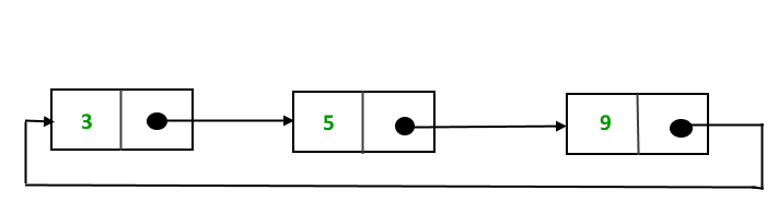
In a linked queue, each node of the queue consists of two parts i.e. data part and the link part. Each element of the queue points to its immediate next element in the memory.
In the linked queue, there are two pointers maintained in the memory i.e. front pointer and rear pointer. The front pointer contains the address of the starting element of the queue while the rear pointer contains the address of the last element of the queue.
Insertion and deletions are performed at rear and front end respectively. If front and rear both are NULL, it indicates that the queue is empty.
The linked representation of queue is shown in the following figure.
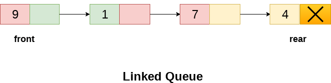
Operation on Linked Queue
There are two basic operations which can be implemented on the linked queues. The operations are Insertion and Deletion.
Insert operation
The insert operation append the queue by adding an element to the end of the queue. The new element will be the last element of the queue.
Firstly, allocate the memory for the new node ptr by using the following statement.
There can be the two scenario of inserting this new node ptr into the linked queue.
In the first scenario, we insert element into an empty queue. In this case, the condition front = NULL becomes true. Now, the new element will be added as the only element of the queue and the next pointer of front and rear pointer both, will point to NULL.
In the second case, the queue contains more than one element. The condition front = NULL becomes false. In this scenario, we need to update the end pointer rear so that the next pointer of rear will point to the new node ptr. Since, this is a linked queue, hence we also need to make the rear pointer point to the newly added node ptr. We also need to make the next pointer of rear point to NULL.
In this way, the element is inserted into the queue. The algorithm and the C implementation is given as follows.
Algorithm
- Step 1: Allocate the space for the new node PTR
- Step 2: SET PTR -> DATA = VAL
- Step 3: IF FRONT = NULL
SET FRONT = REAR = PTR
SET FRONT -> NEXT = REAR -> NEXT = NULL
ELSE
SET REAR -> NEXT = PTR
SET REAR = PTR
SET REAR -> NEXT = NULL
[END OF IF] - Step 4: END
Deletion
Deletion operation removes the element that is first inserted among all the queue elements. Firstly, we need to check either the list is empty or not. The condition front == NULL becomes true if the list is empty, in this case , we simply write underflow on the console and make exit.
Otherwise, we will delete the element that is pointed by the pointer front. For this purpose, copy the node pointed by the front pointer into the pointer ptr. Now, shift the front pointer, point to its next node and free the node pointed by the node ptr. This is done by using the following statements.
The algorithm and C function is given as follows.
Algorithm
- Step 1: IF FRONT = NULL
Write " Underflow "
Go to Step 5
[END OF IF] - Step 2: SET PTR = FRONT
- Step 3: SET FRONT = FRONT -> NEXT
- Step 4: FREE PTR
- Step 5: END
Bubble Sort
In Bubble sort, Each element of the array is compared with its adjacent element. The algorithm processes the list in passes. A list with n elements requires n-1 passes for sorting. Consider an array A of n elements whose elements are to be sorted by using Bubble sort. The algorithm processes like following.
- In Pass 1, A[0] is compared with A[1], A[1] is compared with A[2], A[2] is compared with A[3] and so on. At the end of pass 1, the largest element of the list is placed at the highest index of the list.
- In Pass 2, A[0] is compared with A[1], A[1] is compared with A[2] and so on. At the end of Pass 2 the second largest element of the list is placed at the second highest index of the list.
- In pass n-1, A[0] is compared with A[1], A[1] is compared with A[2] and so on. At the end of this pass. The smallest element of the list is placed at the first index of the list.
Algorithm :
- Step 1: Repeat Step 2 For i = 0 to N-1
- Step 2: Repeat For J = i + 1 to N - I
- Step 3: IF A[J] > A[i]
SWAP A[J] and A[i]
[END OF INNER LOOP]
[END OF OUTER LOOP - Step 4: EXIT
How Bubble Sort Works?
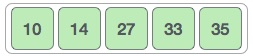
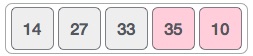
We take an unsorted array for our example. Bubble sort takes Ο(n2) time so we're keeping it short and precise.
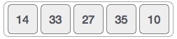
Bubble sort starts with very first two elements, comparing them to check which one is greater.
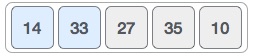
In this case, value 33 is greater than 14, so it is already in sorted locations. Next, we compare 33 with 27.
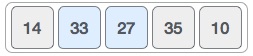
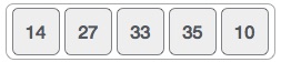
We find that 27 is smaller than 33 and these two values must be swapped.
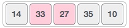
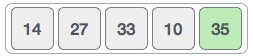
The new array should look like this −
Next we compare 33 and 35. We find that both are in already sorted positions.
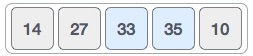
Then we move to the next two values, 35 and 10.
We know then that 10 is smaller 35. Hence they are not sorted.
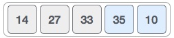
We swap these values. We find that we have reached the end of the array. After one iteration, the array should look like this −
To be precise, we are now showing how an array should look like after each iteration. After the second iteration, it should look like this −
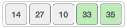
Notice that after each iteration, at least one value moves at the end.
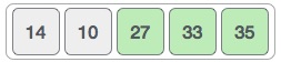
And when there's no swap required, bubble sorts learns that an array is completely sorted.